Lecture 3 — Optimization (Unconstrained & Constrained)

Learning outcomes

By the end of this lecture you will be able to:

• Understand the connection between root finding and the minimization/maximization problem.

• Derive Newton’s method for unconstrained optimization from a Taylor Series Expansion (TSE) and relate it to the root-finding Newton method (replace \(F\) by \(\nabla f\), and \(J\) by \(H\)).

• Formulate optimization problems with the appropriate mathematical notation.

• Understand the difference between constrained and unconstrained optimization.

• Implement a basic optimization algorithm based on Newton’s method using gradients and Hessians.

• Set up curve fitting / parameter estimation as minimization of a sum of squared estimate of errors (SSE).

• Solve constrained problems with scipy.optimize.minimize using gradients when available.

• Recognize when derivative-free optimization (e.g., Nelder–Mead simplex) can be potentially useful and its trade-offs.

1) Motivation (ChemE examples)

• Parameter estimation: infer kinetic or transport parameters from data by minimizing sum of squared estimate of errors (SSE).

• Design & operation: minimize energy/utility cost subject to mass/energy balances and bounds.

• Control & planning: optimize set points or planning variables with constraints

Optimization allows us to choose decision variables optimal values (also known as degrees of freedom) to minimize a scalar objective (with or without constraints).

2) Unconstrained Optimization

Problem Formulation

We want to solve the unconstrained problem

\[ \min_x f(x) \]

In which \(x\) might be a single variable (scalar) or a vector (multivariate). The logic for looking for an optimum point in both cases remains the same. We separate both, so we can properly deal with vectors in the multivariate cases in a mathematical tractable and formal way.

Single-Variable Case (1D)

If we are at a minimum or maximum point of the function (extrema), we have the condition that the derivative is zero:

First-order necessary condition (FONC)
At a candidate optimum \(x^\star\),

\[ f'(x^\star) = 0 \]

This ensures the tangent is flat (horizontal slope).

Second-order conditions (SOC).
Examine the second derivative at \(x^\star\):

• If \(f''(x^\star) > 0\), then \(x^\star\) is a strict local minimum (the curve is convex-up).

• If \(f''(x^\star) < 0\), then \(x^\star\) is a local maximum.

• If \(f''(x^\star) = 0\), the test is inconclusive; higher-order terms or other analysis is needed.

So, in plain english: first derivative = flatness, second derivative = curvature.

Why is that true? optimization is closely tied to root-finding:

• In one variable, finding a minimum of \(f(x)\) requires solving

  \[ f'(x^\star) = 0, \]

  which is just finding the root of the derivative.

• In several variables, we require

  \[ \nabla f(x^\star) = 0, \]

  i.e., solving a system of equations given by the gradient.

This is why Newton’s method for optimization is essentially Newton’s method applied to the gradient.

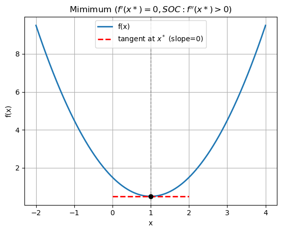
Let’s take a look at this with an actual function.

\[y(x) = (x - 1)^2 + 0.5\]

\[\frac{dy}{dx}=y'(x) = 2(x-1)\]

if

\[ y'(x)=0 \]

then,

\[2(x-1)=0 \leftarrow\rightarrow x=1\]

Taking another derivative, we have

\[\frac{d^2y}{dx^2}=y''(x) = 2 \geq 0 \]

Based on the first and second order conditions, this is a minimum. Let’s plot and see.

import numpy as np

def f(x): 
    return (x - 1.0)**2 + 0.5  

x = np.linspace(-2, 4, 400)
x_star = 1.0  
y = f(x)

import matplotlib.pyplot as plt


plt.plot(x, y, lw=2, label='f(x)')
plt.axvline(x_star, color='gray', ls='--', lw=1)
plt.plot([x_star-1, x_star+1], [f(x_star), f(x_star)], 'r--', lw=2, label='tangent at $x^*$ (slope=0)')
plt.scatter([x_star], [f(x_star)], color='k', zorder=5)
plt.title("Mimimum $(f'(x*)=0, SOC: f''(x*)>0)$")
plt.xlabel("x"); plt.ylabel("f(x)")
plt.legend(); plt.grid(True); plt.show()

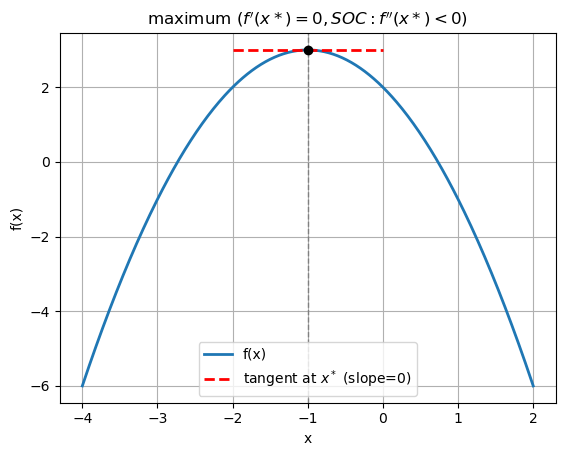
Another example,

\[y(x) = -(x+1)^2 + 3\]

\[y'(x) = 0 = 2(x+1)\leftarrow\rightarrow x = -1\]

\[ y''(x) = -2 \]

Which is a maximum. Let’s check again.

def f2(x): 
    return -(x + 1.0)**2 + 3.0 

x = np.linspace(-4, 2, 400)
x_star = -1.0
y = f2(x)

plt.plot(x, y, lw=2, label='f(x)')
plt.axvline(x_star, color='gray', ls='--', lw=1)
plt.plot([x_star-1, x_star+1], [f2(x_star), f2(x_star)], 'r--', lw=2, label='tangent at $x^*$ (slope=0)')
plt.scatter([x_star], [f2(x_star)], color='k', zorder=5)
plt.title("maximum $(f'(x*)=0, SOC: f''(x*)<0)$")
plt.xlabel("x"); plt.ylabel("f(x)")
plt.legend(); plt.grid(True); plt.show()

Why This Carries Over to Higher Dimensions

In higher dimensions, \(f:\mathbb{R}^n \to \mathbb{R}\), the same geometric intuition applies:

• The gradient \(\nabla f(x)\) generalizes the derivative:

  • In 1D, \(f'(x^\star)=0\) means slope \(=0\).

  • In nD, \(\nabla f(x^\star)=0\) means no slope in any direction.

• The Hessian \(H(x)\) generalizes the second derivative:

  • In 1D, \(f''(x^\star)>0\) means “curved upward.”

  • In nD, \(H(x^\star)\) positive definite means the function curves upward in every direction, hence a strict local minimum.

Thus, the same logic extends naturally: flatness (first order condition) + curvature (second order condition).

Newton’s Method for Optimization via Taylor Series Expansion (TSE)

From Root-Finding to Optimization

In root-finding, we solved

\[f(x) = 0\]

For optimization, the first-order condition says that at a minimizer \(x^\star\) we must have

\[\nabla f(x^\star) = 0\]

So optimization reduces to finding a root of the gradient!

Taylor Expansion of the Gradient

Let \(g(x) = \nabla f(x)\) (the gradient). Expand \(g\) around the current iterate \(x_k\) using a first-order Taylor series:

\[ g(x) \approx g(x_k) + H(x_k)\,(x - x_k), \]

where \(H(x_k) = \nabla^2 f(x_k)\) is the Hessian, which is defined as:

\[\begin{split} H(x) = \nabla^2 f(x) = \begin{bmatrix} \frac{\partial^2 f(x)}{\partial x_1^2} & \frac{\partial^2 f(x)}{\partial x_1 \partial x_2} & \cdots & \frac{\partial^2 f(x)}{\partial x_1 \partial x_n} \\[1.2ex] \frac{\partial^2 f(x)}{\partial x_2 \partial x_1} & \frac{\partial^2 f(x)}{\partial x_2^2} & \cdots & \frac{\partial^2 f(x)}{\partial x_2 \partial x_n} \\[1.2ex] \vdots & \vdots & \ddots & \vdots \\[1.2ex] \frac{\partial^2 f(x)}{\partial x_n \partial x_1} & \frac{\partial^2 f(x)}{\partial x_n \partial x_2} & \cdots & \frac{\partial^2 f(x)}{\partial x_n^2} \end{bmatrix} \end{split}\]

Impose Root Condition on Gradient Function!

At the next iterate \(x_{k+1}\), we want \(g(x_{k+1}) = 0\). Substitute into the expansion:

\[ 0 \approx g(x_k) + H(x_k)\,(x_{k+1} - x_k) \]

Solve for the Newton Step

Rearrange to obtain the Newton step for optimization:

\[ H(x_k)\,(x_{k+1} - x_k) = -\,g(x_k), \]

so

\[ x_{k+1} = x_k - H(x_k)^{-1}\,g(x_k). \]

This mirrors the root-finding Newton step, with the identifications \(F \equiv g\) and \(J \equiv H\).

Single-Variable Special Case

If \(f:\mathbb{R}\to\mathbb{R}\), then \(g(x) = f'(x)\) and \(H(x) = f''(x)\), giving the classic 1D Newton update for optimization:

\[ x_{k+1} = x_k - \frac{f'(x_k)}{f''(x_k)}. \]

How would we implement this as an algorithm?

Pseudocode: Newton’s Method for Optimization

Inputs:

• Objective function \(f(x)\)

• Gradient \(\nabla f(x)\)

• Hessian \(\nabla^2 f(x)\)

• Initial guess \(x_0\)

• Tolerance \(\varepsilon\)

• Maximum iterations \(N_{\text{max}}\)

Algorithm:

1. Set \(k = 0\).

2. Initialize \(x = x_0\).

3. While \(k < N_{\text{max}}\):
   a. Compute gradient \(g = \nabla f(x)\).
   b. If \(\| g \| < \varepsilon\), stop (converged).
   c. Compute Hessian \(H = \nabla^2 f(x)\).
   d. Solve the linear system \(H d = -g\) for the step \(d\).
   e. Update \(x \leftarrow x + d\).
   f. Increment \(k \leftarrow k+1\).

4. Return final point \(x\).

Outputs:

• Approximate minimizer \(x^\ast\)

Optional (diagnosis)

• Gradient norm \(\| g \|\)

• Number of iterations

In actual code, this is how it looks like:

import numpy as np

def newton_min(f, grad, hess, x0, tol=1e-8, max_iter = 50):


    """
    Newton's method for minimization.


    Inputs
    ------

    f: function
        The function we want to minimize.

    grad
        Gradient of the function.
    
    hess
        Hessian of the function.
    
    x0
        Initial estimate.
    
    tol
        Tolerance.
    max_iter
        Max. number of iterations

    Returns
    -------

    x
        approximate minimizer of the function f.
    
    iter
        # of iterations.
    sol
        Value of f(x) at the solution
    
    
    
    """

    x = x0

    for k in range(max_iter):

        H = hess(x)

        eigenvals = np.linalg.eigvals(H)

        if np.any(eigenvals <= 0 ):
            raise ValueError(f"Hessian not positive definite at iteration {k}")
        

        d = np.linalg.inv(H) @ grad(x)
        x_new = x - d

        if np.linalg.norm(grad(x_new), ord = 2) < tol: # Function norm small enough. Stop.
            
            return x_new, k+1, np.abs(f(x_new)), np.linalg.norm(grad(x_new), ord = 2)
        
        if np.linalg.norm((x_new -  x), ord = 2) < 1e-14:

            return x_new, k+1, np.abs(f(x_new)), np.linalg.norm(grad(x_new), ord = 2)
        
        x = x_new

    fx = f(x)
    x = x_new

    raise ValueError(f"Newton's method did not converge after {k+1} iterations;", f"x={x:.6f}, f(x)={fx:.6f}")

We are checking the hessian curvature here and exiting if it’s not positive definite. But this is not exactly how this is handled in large-scale optimization algorithms. We just don’t give up if during an iteration, the curvature is not going towards decrease.

It is beyond of the scope of today’s class, but what actually happens is the solvers are built such that hessian approximations are generated in a way that we will always have a positive curvature (hopefully). One of the techniques employed is Cholesky decomposition.

Unconstrained example (simple convex “bowl”)

Let’s look at this example, visually. $\( f(x,y)=(x-1)^2 + 10\,(y-2)^2,\quad \nabla f(x,y)=\begin{bmatrix}2(x-1)\\ 20(y-2)\end{bmatrix},\quad H=\begin{bmatrix}2&0\\0&20\end{bmatrix}. \)$

import numpy as np
import matplotlib.pyplot as plt
from mpl_toolkits.mplot3d import Axes3D 


def f_xy(v):
    x, y = v
    return (x-1)**2 + 10*(y-2)**2

# Gradient: g(x,y) = [2(x-1), 20(y-2)]
def grad_xy(x, y):
    return np.array([2*(x - 1.0), 20*(y - 2.0)])

# Grid for plotting
x = np.linspace(-1, 3, 200)
y = np.linspace(0, 4, 200)
X, Y = np.meshgrid(x, y)
Z = np.array([[f_xy([xi, yi]) for xi, yi in zip(row_x, row_y)]
              for row_x, row_y in zip(X, Y)])

# 3D Surface Plot 
fig = plt.figure(figsize=(12, 5))
ax1 = fig.add_subplot(1, 2, 1, projection="3d")
surf = ax1.plot_surface(X, Y, Z, cmap="viridis", alpha=0.9, edgecolor="none")
ax1.scatter(1, 2, f_xy([1, 2]), color="r", s=50, label="Solution (1,2)")
ax1.view_init(elev=30, azim=22.5) 
ax1.set_title("Surface of $f(x,y)$")
ax1.set_xlabel("$x$")
ax1.set_ylabel("$y$")
ax1.set_zlabel("$f(x,y)$")
ax1.legend()

# Contour Plot with Gradient Field 
ax2 = fig.add_subplot(1, 2, 2)
contours = ax2.contour(X, Y, Z, levels=20, cmap="viridis")
ax2.clabel(contours, inline=True, fontsize=8)
ax2.plot(1, 2, 'ro', markersize=8, label="Solution (1,2)")

# Sparse grid for vectors to avoid clutter
xs = np.linspace(-1, 3, 17)
ys = np.linspace(0, 4, 17)
XS, YS = np.meshgrid(xs, ys)

# Compute gradient and (negative) gradient for arrows
G = np.array([grad_xy(xi, yi) for xi, yi in zip(XS.ravel(), YS.ravel())])
Ux = G[:, 0].reshape(XS.shape)     # ∇f x-component (uphill)
Uy = G[:, 1].reshape(YS.shape)     # ∇f y-component
Vx = -Ux                           # -∇f (steepest descent)
Vy = -Uy

# Normalize for nicer arrows (optional)
norm = np.sqrt(Ux**2 + Uy**2) + 1e-12
Ux_n = Ux / norm
Uy_n = Uy / norm
Vx_n = Vx / norm
Vy_n = Vy / norm

# Plot both gradient and negative gradient (different styles)
ax2.quiver(XS, YS, Ux_n, Uy_n, color='tab:orange', alpha=0.8, scale=30, width=0.003, label=r"$\nabla f$")
ax2.quiver(XS, YS, Vx_n, Vy_n, color='tab:blue', alpha=0.8, scale=30, width=0.003, label=r"$-\nabla f$")

ax2.set_title(r"Contour of $f(x,y)$ with $\nabla f$ (uphill) and $-\nabla f$ (descent)")
ax2.set_xlabel("$x$")
ax2.set_ylabel("$y$")
ax2.legend()
ax2.axis("equal")

plt.tight_layout()
plt.show()

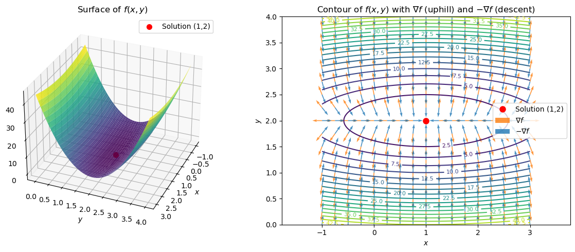
In the figure above we see some important geometrical insight: The negative gradient gives the fastest direction to the minimizer \(x^*\)!

If we solve this, we should get \(x^*=[1,2]\)

def f_xy(v):
    x, y = v
    return (x-1)**2 + 10*(y-2)**2

def g_xy(v):
    x, y = v
    return np.array([2*(x-1), 20*(y-2)])

def H_xy(v):
    return np.array([[2.0, 0.0],
                     [0.0, 20.0]])

x_star, iters, info, norm_grad = newton_min(f_xy, g_xy, H_xy, x0=[-1.0, 4.0])
print("x* =", x_star, "| iters:", iters, "|f(x):", info, "| |gradient|:", norm_grad)

x* = [1. 2.] | iters: 1 |f(x): 0.0 | |gradient|: 0.0

import scipy as sp

?sp.optimize.minimize

Signature:
sp.optimize.minimize(
    fun,
    x0,
    args=(),
    method=None,
    jac=None,
    hess=None,
    hessp=None,
    bounds=None,
    constraints=(),
    tol=None,
    callback=None,
    options=None,
)
Docstring:
Minimization of scalar function of one or more variables.

Parameters
----------
fun : callable
    The objective function to be minimized::

        fun(x, *args) -> float

    where ``x`` is a 1-D array with shape (n,) and ``args``
    is a tuple of the fixed parameters needed to completely
    specify the function.

    Suppose the callable has signature ``f0(x, *my_args, **my_kwargs)``, where
    ``my_args`` and ``my_kwargs`` are required positional and keyword arguments.
    Rather than passing ``f0`` as the callable, wrap it to accept
    only ``x``; e.g., pass ``fun=lambda x: f0(x, *my_args, **my_kwargs)`` as the
    callable, where ``my_args`` (tuple) and ``my_kwargs`` (dict) have been
    gathered before invoking this function.
x0 : ndarray, shape (n,)
    Initial guess. Array of real elements of size (n,),
    where ``n`` is the number of independent variables.
args : tuple, optional
    Extra arguments passed to the objective function and its
    derivatives (`fun`, `jac` and `hess` functions).
method : str or callable, optional
    Type of solver.  Should be one of

    - 'Nelder-Mead' :ref:`(see here) <optimize.minimize-neldermead>`
    - 'Powell'      :ref:`(see here) <optimize.minimize-powell>`
    - 'CG'          :ref:`(see here) <optimize.minimize-cg>`
    - 'BFGS'        :ref:`(see here) <optimize.minimize-bfgs>`
    - 'Newton-CG'   :ref:`(see here) <optimize.minimize-newtoncg>`
    - 'L-BFGS-B'    :ref:`(see here) <optimize.minimize-lbfgsb>`
    - 'TNC'         :ref:`(see here) <optimize.minimize-tnc>`
    - 'COBYLA'      :ref:`(see here) <optimize.minimize-cobyla>`
    - 'COBYQA'      :ref:`(see here) <optimize.minimize-cobyqa>`
    - 'SLSQP'       :ref:`(see here) <optimize.minimize-slsqp>`
    - 'trust-constr':ref:`(see here) <optimize.minimize-trustconstr>`
    - 'dogleg'      :ref:`(see here) <optimize.minimize-dogleg>`
    - 'trust-ncg'   :ref:`(see here) <optimize.minimize-trustncg>`
    - 'trust-exact' :ref:`(see here) <optimize.minimize-trustexact>`
    - 'trust-krylov' :ref:`(see here) <optimize.minimize-trustkrylov>`
    - custom - a callable object, see below for description.

    If not given, chosen to be one of ``BFGS``, ``L-BFGS-B``, ``SLSQP``,
    depending on whether or not the problem has constraints or bounds.
jac : {callable,  '2-point', '3-point', 'cs', bool}, optional
    Method for computing the gradient vector. Only for CG, BFGS,
    Newton-CG, L-BFGS-B, TNC, SLSQP, dogleg, trust-ncg, trust-krylov,
    trust-exact and trust-constr.
    If it is a callable, it should be a function that returns the gradient
    vector::

        jac(x, *args) -> array_like, shape (n,)

    where ``x`` is an array with shape (n,) and ``args`` is a tuple with
    the fixed parameters. If `jac` is a Boolean and is True, `fun` is
    assumed to return a tuple ``(f, g)`` containing the objective
    function and the gradient.
    Methods 'Newton-CG', 'trust-ncg', 'dogleg', 'trust-exact', and
    'trust-krylov' require that either a callable be supplied, or that
    `fun` return the objective and gradient.
    If None or False, the gradient will be estimated using 2-point finite
    difference estimation with an absolute step size.
    Alternatively, the keywords  {'2-point', '3-point', 'cs'} can be used
    to select a finite difference scheme for numerical estimation of the
    gradient with a relative step size. These finite difference schemes
    obey any specified `bounds`.
hess : {callable, '2-point', '3-point', 'cs', HessianUpdateStrategy}, optional
    Method for computing the Hessian matrix. Only for Newton-CG, dogleg,
    trust-ncg, trust-krylov, trust-exact and trust-constr.
    If it is callable, it should return the Hessian matrix::

        hess(x, *args) -> {LinearOperator, spmatrix, array}, (n, n)

    where ``x`` is a (n,) ndarray and ``args`` is a tuple with the fixed
    parameters.
    The keywords {'2-point', '3-point', 'cs'} can also be used to select
    a finite difference scheme for numerical estimation of the hessian.
    Alternatively, objects implementing the `HessianUpdateStrategy`
    interface can be used to approximate the Hessian. Available
    quasi-Newton methods implementing this interface are:

    - `BFGS`
    - `SR1`

    Not all of the options are available for each of the methods; for
    availability refer to the notes.
hessp : callable, optional
    Hessian of objective function times an arbitrary vector p. Only for
    Newton-CG, trust-ncg, trust-krylov, trust-constr.
    Only one of `hessp` or `hess` needs to be given. If `hess` is
    provided, then `hessp` will be ignored. `hessp` must compute the
    Hessian times an arbitrary vector::

        hessp(x, p, *args) ->  ndarray shape (n,)

    where ``x`` is a (n,) ndarray, ``p`` is an arbitrary vector with
    dimension (n,) and ``args`` is a tuple with the fixed
    parameters.
bounds : sequence or `Bounds`, optional
    Bounds on variables for Nelder-Mead, L-BFGS-B, TNC, SLSQP, Powell,
    trust-constr, COBYLA, and COBYQA methods. There are two ways to specify
    the bounds:

    1. Instance of `Bounds` class.
    2. Sequence of ``(min, max)`` pairs for each element in `x`. None
       is used to specify no bound.

constraints : {Constraint, dict} or List of {Constraint, dict}, optional
    Constraints definition. Only for COBYLA, COBYQA, SLSQP and trust-constr.

    Constraints for 'trust-constr', 'cobyqa', and 'cobyla' are defined as a single
    object or a list of objects specifying constraints to the optimization problem.
    Available constraints are:

    - `LinearConstraint`
    - `NonlinearConstraint`

    Constraints for COBYLA, SLSQP are defined as a list of dictionaries.
    Each dictionary with fields:

    type : str
        Constraint type: 'eq' for equality, 'ineq' for inequality.
    fun : callable
        The function defining the constraint.
    jac : callable, optional
        The Jacobian of `fun` (only for SLSQP).
    args : sequence, optional
        Extra arguments to be passed to the function and Jacobian.

    Equality constraint means that the constraint function result is to
    be zero whereas inequality means that it is to be non-negative.
    Note that COBYLA only supports inequality constraints.

tol : float, optional
    Tolerance for termination. When `tol` is specified, the selected
    minimization algorithm sets some relevant solver-specific tolerance(s)
    equal to `tol`. For detailed control, use solver-specific
    options.
options : dict, optional
    A dictionary of solver options. All methods except `TNC` accept the
    following generic options:

    maxiter : int
        Maximum number of iterations to perform. Depending on the
        method each iteration may use several function evaluations.

        For `TNC` use `maxfun` instead of `maxiter`.
    disp : bool
        Set to True to print convergence messages.

    For method-specific options, see :func:`show_options()`.
callback : callable, optional
    A callable called after each iteration.

    All methods except TNC and SLSQP support a callable with
    the signature::

        callback(intermediate_result: OptimizeResult)

    where ``intermediate_result`` is a keyword parameter containing an
    `OptimizeResult` with attributes ``x`` and ``fun``, the present values
    of the parameter vector and objective function. Not all attributes of
    `OptimizeResult` may be present. The name of the parameter must be
    ``intermediate_result`` for the callback to be passed an `OptimizeResult`.
    These methods will also terminate if the callback raises ``StopIteration``.

    All methods except trust-constr (also) support a signature like::

        callback(xk)

    where ``xk`` is the current parameter vector.

    Introspection is used to determine which of the signatures above to
    invoke.

Returns
-------
res : OptimizeResult
    The optimization result represented as a ``OptimizeResult`` object.
    Important attributes are: ``x`` the solution array, ``success`` a
    Boolean flag indicating if the optimizer exited successfully and
    ``message`` which describes the cause of the termination. See
    `OptimizeResult` for a description of other attributes.

See also
--------
minimize_scalar : Interface to minimization algorithms for scalar
    univariate functions
show_options : Additional options accepted by the solvers

Notes
-----
This section describes the available solvers that can be selected by the
'method' parameter. The default method is *BFGS*.

**Unconstrained minimization**

Method :ref:`CG <optimize.minimize-cg>` uses a nonlinear conjugate
gradient algorithm by Polak and Ribiere, a variant of the
Fletcher-Reeves method described in [5]_ pp.120-122. Only the
first derivatives are used.

Method :ref:`BFGS <optimize.minimize-bfgs>` uses the quasi-Newton
method of Broyden, Fletcher, Goldfarb, and Shanno (BFGS) [5]_
pp. 136. It uses the first derivatives only. BFGS has proven good
performance even for non-smooth optimizations. This method also
returns an approximation of the Hessian inverse, stored as
`hess_inv` in the OptimizeResult object.

Method :ref:`Newton-CG <optimize.minimize-newtoncg>` uses a
Newton-CG algorithm [5]_ pp. 168 (also known as the truncated
Newton method). It uses a CG method to the compute the search
direction. See also *TNC* method for a box-constrained
minimization with a similar algorithm. Suitable for large-scale
problems.

Method :ref:`dogleg <optimize.minimize-dogleg>` uses the dog-leg
trust-region algorithm [5]_ for unconstrained minimization. This
algorithm requires the gradient and Hessian; furthermore the
Hessian is required to be positive definite.

Method :ref:`trust-ncg <optimize.minimize-trustncg>` uses the
Newton conjugate gradient trust-region algorithm [5]_ for
unconstrained minimization. This algorithm requires the gradient
and either the Hessian or a function that computes the product of
the Hessian with a given vector. Suitable for large-scale problems.

Method :ref:`trust-krylov <optimize.minimize-trustkrylov>` uses
the Newton GLTR trust-region algorithm [14]_, [15]_ for unconstrained
minimization. This algorithm requires the gradient
and either the Hessian or a function that computes the product of
the Hessian with a given vector. Suitable for large-scale problems.
On indefinite problems it requires usually less iterations than the
`trust-ncg` method and is recommended for medium and large-scale problems.

Method :ref:`trust-exact <optimize.minimize-trustexact>`
is a trust-region method for unconstrained minimization in which
quadratic subproblems are solved almost exactly [13]_. This
algorithm requires the gradient and the Hessian (which is
*not* required to be positive definite). It is, in many
situations, the Newton method to converge in fewer iterations
and the most recommended for small and medium-size problems.

**Bound-Constrained minimization**

Method :ref:`Nelder-Mead <optimize.minimize-neldermead>` uses the
Simplex algorithm [1]_, [2]_. This algorithm is robust in many
applications. However, if numerical computation of derivative can be
trusted, other algorithms using the first and/or second derivatives
information might be preferred for their better performance in
general.

Method :ref:`L-BFGS-B <optimize.minimize-lbfgsb>` uses the L-BFGS-B
algorithm [6]_, [7]_ for bound constrained minimization.

Method :ref:`Powell <optimize.minimize-powell>` is a modification
of Powell's method [3]_, [4]_ which is a conjugate direction
method. It performs sequential one-dimensional minimizations along
each vector of the directions set (`direc` field in `options` and
`info`), which is updated at each iteration of the main
minimization loop. The function need not be differentiable, and no
derivatives are taken. If bounds are not provided, then an
unbounded line search will be used. If bounds are provided and
the initial guess is within the bounds, then every function
evaluation throughout the minimization procedure will be within
the bounds. If bounds are provided, the initial guess is outside
the bounds, and `direc` is full rank (default has full rank), then
some function evaluations during the first iteration may be
outside the bounds, but every function evaluation after the first
iteration will be within the bounds. If `direc` is not full rank,
then some parameters may not be optimized and the solution is not
guaranteed to be within the bounds.

Method :ref:`TNC <optimize.minimize-tnc>` uses a truncated Newton
algorithm [5]_, [8]_ to minimize a function with variables subject
to bounds. This algorithm uses gradient information; it is also
called Newton Conjugate-Gradient. It differs from the *Newton-CG*
method described above as it wraps a C implementation and allows
each variable to be given upper and lower bounds.

**Constrained Minimization**

Method :ref:`COBYLA <optimize.minimize-cobyla>` uses the PRIMA
implementation [19]_ of the
Constrained Optimization BY Linear Approximation (COBYLA) method
[9]_, [10]_, [11]_. The algorithm is based on linear
approximations to the objective function and each constraint.

Method :ref:`COBYQA <optimize.minimize-cobyqa>` uses the Constrained
Optimization BY Quadratic Approximations (COBYQA) method [18]_. The
algorithm is a derivative-free trust-region SQP method based on quadratic
approximations to the objective function and each nonlinear constraint. The
bounds are treated as unrelaxable constraints, in the sense that the
algorithm always respects them throughout the optimization process.

Method :ref:`SLSQP <optimize.minimize-slsqp>` uses Sequential
Least SQuares Programming to minimize a function of several
variables with any combination of bounds, equality and inequality
constraints. The method wraps the SLSQP Optimization subroutine
originally implemented by Dieter Kraft [12]_. Note that the
wrapper handles infinite values in bounds by converting them into
large floating values.

Method :ref:`trust-constr <optimize.minimize-trustconstr>` is a
trust-region algorithm for constrained optimization. It switches
between two implementations depending on the problem definition.
It is the most versatile constrained minimization algorithm
implemented in SciPy and the most appropriate for large-scale problems.
For equality constrained problems it is an implementation of Byrd-Omojokun
Trust-Region SQP method described in [17]_ and in [5]_, p. 549. When
inequality constraints are imposed as well, it switches to the trust-region
interior point method described in [16]_. This interior point algorithm,
in turn, solves inequality constraints by introducing slack variables
and solving a sequence of equality-constrained barrier problems
for progressively smaller values of the barrier parameter.
The previously described equality constrained SQP method is
used to solve the subproblems with increasing levels of accuracy
as the iterate gets closer to a solution.

**Finite-Difference Options**

For Method :ref:`trust-constr <optimize.minimize-trustconstr>`
the gradient and the Hessian may be approximated using
three finite-difference schemes: {'2-point', '3-point', 'cs'}.
The scheme 'cs' is, potentially, the most accurate but it
requires the function to correctly handle complex inputs and to
be differentiable in the complex plane. The scheme '3-point' is more
accurate than '2-point' but requires twice as many operations. If the
gradient is estimated via finite-differences the Hessian must be
estimated using one of the quasi-Newton strategies.

**Method specific options for the** `hess` **keyword**

+--------------+------+----------+-------------------------+-----+
| method/Hess  | None | callable | '2-point/'3-point'/'cs' | HUS |
+==============+======+==========+=========================+=====+
| Newton-CG    | x    | (n, n)   | x                       | x   |
|              |      | LO       |                         |     |
+--------------+------+----------+-------------------------+-----+
| dogleg       |      | (n, n)   |                         |     |
+--------------+------+----------+-------------------------+-----+
| trust-ncg    |      | (n, n)   | x                       | x   |
+--------------+------+----------+-------------------------+-----+
| trust-krylov |      | (n, n)   | x                       | x   |
+--------------+------+----------+-------------------------+-----+
| trust-exact  |      | (n, n)   |                         |     |
+--------------+------+----------+-------------------------+-----+
| trust-constr | x    | (n, n)   |  x                      | x   |
|              |      | LO       |                         |     |
|              |      | sp       |                         |     |
+--------------+------+----------+-------------------------+-----+

where LO=LinearOperator, sp=Sparse matrix, HUS=HessianUpdateStrategy

**Custom minimizers**

It may be useful to pass a custom minimization method, for example
when using a frontend to this method such as `scipy.optimize.basinhopping`
or a different library.  You can simply pass a callable as the ``method``
parameter.

The callable is called as ``method(fun, x0, args, **kwargs, **options)``
where ``kwargs`` corresponds to any other parameters passed to `minimize`
(such as `callback`, `hess`, etc.), except the `options` dict, which has
its contents also passed as `method` parameters pair by pair.  Also, if
`jac` has been passed as a bool type, `jac` and `fun` are mangled so that
`fun` returns just the function values and `jac` is converted to a function
returning the Jacobian.  The method shall return an `OptimizeResult`
object.

The provided `method` callable must be able to accept (and possibly ignore)
arbitrary parameters; the set of parameters accepted by `minimize` may
expand in future versions and then these parameters will be passed to
the method.  You can find an example in the scipy.optimize tutorial.

References
----------
.. [1] Nelder, J A, and R Mead. 1965. A Simplex Method for Function
    Minimization. The Computer Journal 7: 308-13.
.. [2] Wright M H. 1996. Direct search methods: Once scorned, now
    respectable, in Numerical Analysis 1995: Proceedings of the 1995
    Dundee Biennial Conference in Numerical Analysis (Eds. D F
    Griffiths and G A Watson). Addison Wesley Longman, Harlow, UK.
    191-208.
.. [3] Powell, M J D. 1964. An efficient method for finding the minimum of
   a function of several variables without calculating derivatives. The
   Computer Journal 7: 155-162.
.. [4] Press W, S A Teukolsky, W T Vetterling and B P Flannery.
   Numerical Recipes (any edition), Cambridge University Press.
.. [5] Nocedal, J, and S J Wright. 2006. Numerical Optimization.
   Springer New York.
.. [6] Byrd, R H and P Lu and J. Nocedal. 1995. A Limited Memory
   Algorithm for Bound Constrained Optimization. SIAM Journal on
   Scientific and Statistical Computing 16 (5): 1190-1208.
.. [7] Zhu, C and R H Byrd and J Nocedal. 1997. L-BFGS-B: Algorithm
   778: L-BFGS-B, FORTRAN routines for large scale bound constrained
   optimization. ACM Transactions on Mathematical Software 23 (4):
   550-560.
.. [8] Nash, S G. Newton-Type Minimization Via the Lanczos Method.
   1984. SIAM Journal of Numerical Analysis 21: 770-778.
.. [9] Powell, M J D. A direct search optimization method that models
   the objective and constraint functions by linear interpolation.
   1994. Advances in Optimization and Numerical Analysis, eds. S. Gomez
   and J-P Hennart, Kluwer Academic (Dordrecht), 51-67.
.. [10] Powell M J D. Direct search algorithms for optimization
   calculations. 1998. Acta Numerica 7: 287-336.
.. [11] Powell M J D. A view of algorithms for optimization without
   derivatives. 2007.Cambridge University Technical Report DAMTP
   2007/NA03
.. [12] Kraft, D. A software package for sequential quadratic
   programming. 1988. Tech. Rep. DFVLR-FB 88-28, DLR German Aerospace
   Center -- Institute for Flight Mechanics, Koln, Germany.
.. [13] Conn, A. R., Gould, N. I., and Toint, P. L.
   Trust region methods. 2000. Siam. pp. 169-200.
.. [14] F. Lenders, C. Kirches, A. Potschka: "trlib: A vector-free
   implementation of the GLTR method for iterative solution of
   the trust region problem", :arxiv:`1611.04718`
.. [15] N. Gould, S. Lucidi, M. Roma, P. Toint: "Solving the
   Trust-Region Subproblem using the Lanczos Method",
   SIAM J. Optim., 9(2), 504--525, (1999).
.. [16] Byrd, Richard H., Mary E. Hribar, and Jorge Nocedal. 1999.
    An interior point algorithm for large-scale nonlinear  programming.
    SIAM Journal on Optimization 9.4: 877-900.
.. [17] Lalee, Marucha, Jorge Nocedal, and Todd Plantenga. 1998. On the
    implementation of an algorithm for large-scale equality constrained
    optimization. SIAM Journal on Optimization 8.3: 682-706.
.. [18] Ragonneau, T. M. *Model-Based Derivative-Free Optimization Methods
    and Software*. PhD thesis, Department of Applied Mathematics, The Hong
    Kong Polytechnic University, Hong Kong, China, 2022. URL:
    https://theses.lib.polyu.edu.hk/handle/200/12294.
.. [19] Zhang, Z. "PRIMA: Reference Implementation for Powell's Methods with
    Modernization and Amelioration", https://www.libprima.net,
    :doi:`10.5281/zenodo.8052654`
.. [20] Karush-Kuhn-Tucker conditions,
    https://en.wikipedia.org/wiki/Karush%E2%80%93Kuhn%E2%80%93Tucker_conditions

Examples
--------
Let us consider the problem of minimizing the Rosenbrock function. This
function (and its respective derivatives) is implemented in `rosen`
(resp. `rosen_der`, `rosen_hess`) in the `scipy.optimize`.

>>> from scipy.optimize import minimize, rosen, rosen_der

A simple application of the *Nelder-Mead* method is:

>>> x0 = [1.3, 0.7, 0.8, 1.9, 1.2]
>>> res = minimize(rosen, x0, method='Nelder-Mead', tol=1e-6)
>>> res.x
array([ 1.,  1.,  1.,  1.,  1.])

Now using the *BFGS* algorithm, using the first derivative and a few
options:

>>> res = minimize(rosen, x0, method='BFGS', jac=rosen_der,
...                options={'gtol': 1e-6, 'disp': True})
Optimization terminated successfully.
         Current function value: 0.000000
         Iterations: 26
         Function evaluations: 31
         Gradient evaluations: 31
>>> res.x
array([ 1.,  1.,  1.,  1.,  1.])
>>> print(res.message)
Optimization terminated successfully.
>>> res.hess_inv
array([
    [ 0.00749589,  0.01255155,  0.02396251,  0.04750988,  0.09495377],  # may vary
    [ 0.01255155,  0.02510441,  0.04794055,  0.09502834,  0.18996269],
    [ 0.02396251,  0.04794055,  0.09631614,  0.19092151,  0.38165151],
    [ 0.04750988,  0.09502834,  0.19092151,  0.38341252,  0.7664427 ],
    [ 0.09495377,  0.18996269,  0.38165151,  0.7664427,   1.53713523]
])

Next, consider a minimization problem with several constraints (namely
Example 16.4 from [5]_). The objective function is:

>>> fun = lambda x: (x[0] - 1)**2 + (x[1] - 2.5)**2

There are three constraints defined as:

>>> cons = ({'type': 'ineq', 'fun': lambda x:  x[0] - 2 * x[1] + 2},
...         {'type': 'ineq', 'fun': lambda x: -x[0] - 2 * x[1] + 6},
...         {'type': 'ineq', 'fun': lambda x: -x[0] + 2 * x[1] + 2})

And variables must be positive, hence the following bounds:

>>> bnds = ((0, None), (0, None))

The optimization problem is solved using the SLSQP method as:

>>> res = minimize(fun, (2, 0), method='SLSQP', bounds=bnds, constraints=cons)

It should converge to the theoretical solution ``[1.4 ,1.7]``. *SLSQP* also
returns the multipliers that are used in the solution of the problem. These
multipliers, when the problem constraints are linear, can be thought of as the
Karush-Kuhn-Tucker (KKT) multipliers, which are a generalization
of Lagrange multipliers to inequality-constrained optimization problems ([20]_).

Notice that at the solution, the first constraint is active. Let's evaluate the
function at solution:

>>> cons[0]['fun'](res.x)
np.float64(1.4901224698604665e-09)

Also, notice that at optimality there is a non-zero multiplier:

>>> res.multipliers
array([0.8, 0. , 0. ])

This can be understood as the local sensitivity of the optimal value of the
objective function with respect to changes in the first constraint. If we
tighten the constraint by a small amount ``eps``:

>>> eps = 0.01
>>> cons[0]['fun'] = lambda x: x[0] - 2 * x[1] + 2 - eps

we expect the optimal value of the objective function to increase by
approximately ``eps * res.multipliers[0]``:

>>> eps * res.multipliers[0]  # Expected change in f0
np.float64(0.008000000027153205)
>>> f0 = res.fun  # Keep track of the previous optimal value
>>> res = minimize(fun, (2, 0), method='SLSQP', bounds=bnds, constraints=cons)
>>> f1 = res.fun  # New optimal value
>>> f1 - f0
np.float64(0.008019998807885509)
File:      /opt/anaconda3/envs/numerical/lib/python3.13/site-packages/scipy/optimize/_minimize.py
Type:      function

import scipy as sp 
x0=[-1.0, 4.0]

solution = sp.optimize.minimize(fun=f_xy, x0=x0, jac=g_xy, hess=H_xy, method='Newton-CG')


print(solution)

 message: Optimization terminated successfully.
 success: True
  status: 0
     fun: 4.930380657631324e-32
       x: [ 1.000e+00  2.000e+00]
     nit: 3
     jac: [ 4.441e-16  0.000e+00]
    nfev: 3
    njev: 3
    nhev: 3

Not providing the gradient gives:

solution = sp.optimize.minimize(fun=f_xy, x0=x0)
print(solution)

  message: Optimization terminated successfully.
  success: True
   status: 0
      fun: 2.2851873995774238e-12
        x: [ 1.000e+00  2.000e+00]
      nit: 7
      jac: [ 1.724e-06  8.036e-06]
 hess_inv: [[ 5.034e-01  1.591e-03]
            [ 1.591e-03  5.074e-02]]
     nfev: 24
     njev: 8

It takes more iterations to reach to the same answer!

3) Curve fitting / parameter estimation as optimization – Sum of Squared Estimate of Errors (SSE)

Given data \(\{x_i, y_i\}\) and a model \(\hat y(x;\theta)\), estimate parameters \(\theta\) by solving the following optimization problem:

\[ \min_\theta\ \text{SSE}(\theta)=\sum_{i=1}^m \big(y_i-\hat y(x_i;\theta)\big)^2 \]

In this case, our degrees of freedom (variables the optimizer manipulates to minimize the error between experimental data and the model predictions) are the parameters we want to estimate!

Let’s look at a simple example.

First-order batch reactor profile: \(\ \hat C(t;k)=C_0 e^{-k t}\)

and we want to determine \(k\). The SSE is defined, as well as the Gradient and the Hessian (since the only variable here is \(k\), these are merely first and second order single-variable derivatives.)

\[ \begin{align}\begin{aligned}\begin{split} \text{SSE}(k)=\sum_i\big(C_i - C_0 e^{-k t_i}\big)^2,\qquad \\\end{split}\\\frac{d\,\text{SSE}}{dk} =2\sum_i \big(C_i-\hat C_i\big)\, t_i\,\hat C_i,\ \ \end{aligned}\end{align} \]

\[ \frac{d^2\,\text{SSE}}{dk^2} =2\sum_i \left[ (t_i \hat C_i)^2 - (C_i-\hat C_i)\,t_i^2\,\hat C_i \right], \qquad \hat C_i = C_0 e^{-k t_i} \]

In our example, I intentionally added noise to the synthetic data, as a way to mimic real data that is noisy. Hence, the value of \(k\) we are going to obtain is not exactly the same when compared against the real value. This is very common in chemical engineering: We estimate parameters for our models using experimental data all the time, and they are, most likely, not \(100\%\) accurate, as experiments (and experimental data) contain noise/randomnes.

Anyway, let’s solve this by minimizing the SSE with scipy.optimize.minimize

import numpy as np
import matplotlib.pyplot as plt
from scipy.optimize import minimize

# synthetic data
t = np.array([0., 1., 2., 3., 4., 5.])
C0 = 1.0
k_true = 0.6
C_true = C0 * np.exp(-k_true * t)

# adding some noise
np.random.seed(42) 
noise_level = 0.05 
C = C_true + noise_level * np.random.randn(t.size)

# objective, gradient, hessian
def SSE(k):
    Chat = C0 * np.exp(-k * t)
    return np.sum((C - Chat)**2)

def dSSE_dk(k):
    Chat = C0 * np.exp(-k * t)
    grad = 2.0 * np.sum((C - Chat) * t * Chat)
    return np.array([grad])

def d2SSE_dk2(k):
    Chat = C0 * np.exp(-k * t)
    term1 = (t * Chat)**2
    term2 = (C - Chat) * (t**2 * Chat)
    hess = 2.0 * np.sum(term1 - term2)
    return np.array([[hess]])


# Solution using scipy
sol = minimize(SSE, x0=0.2, jac=dSSE_dk, hess=d2SSE_dk2, method='trust-exact')

k_hat = sol.x[0]

print('Using Scipy:')
print(sol)
print("Estimated k =", k_hat)
print('-----------------------------------------------------------------------------------------------')
# Solution using our Newton's method.


k_hat_newton, iters, info, norm_grad = newton_min(SSE, dSSE_dk, d2SSE_dk2, x0=0.2)

print("Using Our Newton's method:")
print("k_hat =", k_hat_newton, "| iters:", iters, "|f(x):", info, "| |gradient|:", norm_grad)

print("Estimated k =", k_hat)
print('-----------------------------------------------------------------------------------------------')
# fitted curve
C_fit = C0 * np.exp(-k_hat * t)

# plot
plt.figure(figsize=(6,4))
plt.scatter(t, C, color="red", label="Noisy data", zorder=3)
plt.plot(t, C_true, "k--", label="True model (k=0.6)")
plt.plot(t, C_fit, "b-", label=f"Fitted model (k={k_hat:.3f})")
plt.xlabel("t")
plt.ylabel("C(t)")
plt.legend()
plt.grid(True)
plt.show()

Using Scipy:
 message: Optimization terminated successfully.
 success: True
  status: 0
     fun: 0.005832625399270045
       x: [ 5.598e-01]
     nit: 6
     jac: [-2.527e-07]
    nfev: 7
    njev: 7
    nhev: 7
    hess: [[ 2.673e+00]]
Estimated k = 0.5598385750717667
-----------------------------------------------------------------------------------------------
Using Our Newton's method:
k_hat = [0.55983867] | iters: 7 |f(x): 0.0058326253992581015 | |gradient|: 8.935213680061338e-14
Estimated k = 0.5598385750717667
-----------------------------------------------------------------------------------------------

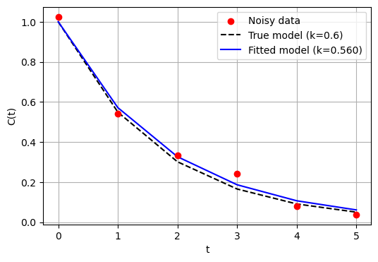
You can see that we got pretty close to the real value used in the model (0.6). But there is some error.

4) Constrained optimization with scipy.optimize.minimize

It is common that we need to find an optimal solution subject to some mathematical relationship that represents what we call a constraint. These constraints in chemical engineering sometimes appear due to physical limitations of equipment, economic profitability or even safety regulations.

For example, the operating temperature of a chemical reactor should not surpass a certain safe value, or the physical dimensions of a distillation column are limited by the economics, or the purity of a product in a chemical plant has to be above a certain value. These are all examples of constraints. Yet, we still need to try to find optimal solutions of such examples that are described mathematically. Let’s take a look at the problem form:

\[\begin{split} \min_{x\in\mathbb{R}^n} f(x)\quad \\ \text{s.t.}\\ \;\; c(x)=0 \quad \\ g(x)\le 0\ \\ x_{l} < x < x_{u} \end{split}\]

You may see this in more details in your next courses, but the gist of the formulation above is that the constraints \(c(x)\) and \(g(x)\) and the objective function \(f(x)\) are rewritten such that we can use our knowledge about unconstrained optimization to solve the constrained optimization problem. We build a function called the Lagrangian, which assembles the constraints and the objective function together:

\[ \mathcal{L}\left(x, \lambda_1, \lambda_2\right)=f(x) + \lambda_1 c(x) + \lambda_2 g(x) \]

And we solve this problem instead. This is what scipy.optimize.minimize is doing under the hood.

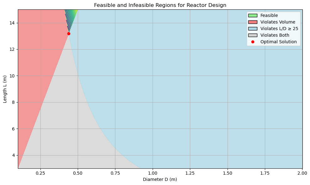
Example – Minimizing Surface Area of a Plug-flow Reactor

Let’s take a look at an example. Say you are given the task of calculating the minimum surface area necessary to manufacture a plug-flow reactor (PFR). Simultaneously, you are given the information that there is a minimum volume that the reactor should have, so the reaction is profitable (i.e., \(2m^3\)). Lastly, to ensure that this PFR actually follows the plug-flow assumption, you need to have the length-to-diameter ration of at least 30.

This translates mathematically as the following problem:

\[\begin{split} \begin{aligned} \min_{D,L}\quad & A(D,L) = \pi D L + \tfrac{\pi}{2} D^{2} \\ \text{s.t.}\quad & \frac{\pi D^{2}}{4}\,L \;\ge\; 2,\\ & \frac{L}{D} \;\ge\; 30,\\ & D_{\min} \le D \le D_{\max},\;\; \\ & L_{\min} \le L \le L_{\max} \end{aligned} \end{split}\]

import numpy as np
from scipy.optimize import minimize

# Objective function: surface area A = pi*D*L + 0.5*pi*D^2
def surface_area(x):
    D, L = x  # D and L in meters, unpacking the vector x appropriately.
    return np.pi * (D * L + 0.5 * D**2)

# Constraint 1: volume must be >= 2.0 m³
def volume_constraint(x):
    D, L = x # D and L in meters, unpacking the vector x appropriately.
    V = (np.pi * D**2 / 4) * L
    return V - 2.0  # must be >= 0

# Constraint 2: L/D >= 30  --> L - 30D >= 0
def plug_flow_constraint(x):
    D, L = x
    constraint_expression = L - 30 * D
    return  constraint_expression # must be >= 0

# Bounds for D and L (in meters)
bounds_list = [(0.1, 2.0), 
               (3.0, 15.0)]  # (D_min, D_max), (L_min, L_max)

# Constraints list
constraints_list = [
    {'type': 'ineq', 'fun': volume_constraint},
    {'type': 'ineq', 'fun': plug_flow_constraint}
]

# Initial guess
x0 = [0.5, 6.0]

# Run optimization
result = minimize(surface_area, 
                  x0, 
                  bounds=bounds_list, 
                  constraints=constraints_list)

# Display results
if result.success:
    D_opt, L_opt = result.x
    A_opt = surface_area([D_opt, L_opt])
    V_opt = (np.pi * D_opt**2 / 4) * L_opt
    L_by_D = L_opt / D_opt

    print("Optimization successful!")
    print(f"Optimal Diameter D: {D_opt:.3f} m")
    print(f"Optimal Length   L: {L_opt:.3f} m")
    print(f"Resulting Volume : {V_opt:.3f} m³")
    print(f"L/D ratio        : {L_by_D:.2f}")
    print(f"Minimum Surface Area: {A_opt:.3f} m²")
else:
    print("Optimization failed.")
    print(result.message)

Optimization successful!
Optimal Diameter D: 0.439 m
Optimal Length   L: 13.184 m
Resulting Volume : 2.000 m³
L/D ratio        : 30.00
Minimum Surface Area: 18.507 m²

Let’s plot the feasible and infeasible regions for this problem and check if we got a solution…

import matplotlib.pyplot as plt
from matplotlib.patches import Patch

# Create grid based on bounds
D_vals = np.linspace(0.1, 2.0, 3000)
L_vals = np.linspace(3.0, 15.0, 3000)
D_grid, L_grid = np.meshgrid(D_vals, L_vals)

# Recalculate surface area, volume, and L/D
A_grid = np.pi * (D_grid * L_grid + 0.5 * D_grid**2)
V_grid = (np.pi * D_grid**2 / 4) * L_grid
L_by_D_grid = L_grid / D_grid

# Classify feasibility
feasible = (V_grid >= 2.0) & (L_by_D_grid >= 30)
vol_only = (V_grid < 2.0) & (L_by_D_grid >= 30)
ld_only = (V_grid >= 2.0) & (L_by_D_grid < 30)
both_violated = (V_grid < 2.0) & (L_by_D_grid < 30)

# Start plot
plt.figure(figsize=(10, 6))

# Shaded regions
plt.contourf(D_grid, L_grid, both_violated, levels=[0.5, 1], colors=['lightgray'], alpha=0.8)
plt.contourf(D_grid, L_grid, vol_only, levels=[0.5, 1], colors=['lightcoral'], alpha=0.8)
plt.contourf(D_grid, L_grid, ld_only, levels=[0.5, 1], colors=['lightblue'], alpha=0.8)
plt.contourf(D_grid, L_grid, feasible, levels=[0.5, 1], colors=['lightgreen'], alpha=0.8)

# Surface area contours over feasible region only
A_feasible = np.ma.masked_where(~feasible, A_grid)
contour = plt.contour(D_grid, L_grid, A_feasible, levels=20, cmap='viridis')

# Optimal solution point
plt.plot(D_opt, L_opt, 'ro', label='Optimal Solution')

# Labels and legend
plt.xlabel('Diameter D (m)')
plt.ylabel('Length L (m)')
plt.title('Feasible and Infeasible Regions for Reactor Design')
plt.grid(True)

# Custom legend
legend_elements = [
    Patch(facecolor='lightgreen', edgecolor='black', label='Feasible'),
    Patch(facecolor='lightcoral', edgecolor='black', label='Violates Volume'),
    Patch(facecolor='lightblue', edgecolor='black', label='Violates L/D ≥ 25'),
    Patch(facecolor='lightgray', edgecolor='black', label='Violates Both'),
    plt.Line2D([0], [0], marker='o', color='w', label='Optimal Solution',
               markerfacecolor='red', markersize=8)
]
plt.legend(handles=legend_elements, loc='upper right')

plt.tight_layout()
plt.show()

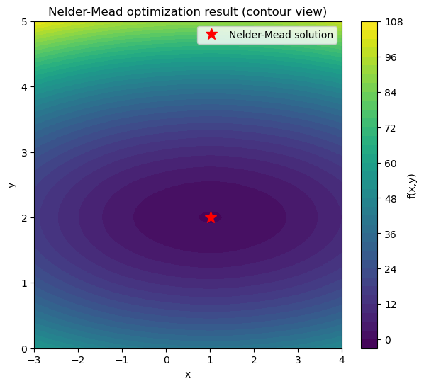
5) Derivative-free optimization (quick note)

When the function we are trying to optimize (\(f\)) is noisy, discontinuous, or nonsmooth, gradients/Hessians can be unreliable.
Nelder–Mead (simplex search) in scipy.optimize.minimize uses only function values — robust to noise but slower and can stagnate in higher dimensions. But sometimes, it can be a viable option.

\[f(x,y) = (x-1)^2 + 10\,(y-2)^2 + 0.05\cos(3x) + 0.05\sin(2y)\]

# Nelder–Mead demo (derivative-free)
def f_nm(v):
    x, y = v
    return (x-1)**2 + 10*(y-2)**2 + 0.05*np.cos(3*x) + 0.05*np.sin(2*y)


res_nm = minimize(f_nm, 
                  x0=[-2.0, 4.0], 
                  method='Nelder-Mead',
                  options={'xatol':1e-8, 'fatol':1e-8, 'maxiter':2000})


print("Nelder-Mead:", res_nm.x, "| nit:", res_nm.nit, "| success:", res_nm.success)

Nelder-Mead: [1.00865317 2.0032436 ] | nit: 90 | success: True

Running scipy.optimize.minimize with default options.

res_defaults = minimize(f_nm, x0=[-2.0, 4.0])

print("scipy default:", res_defaults.x, "| nit:", res_defaults.nit, "| success:", res_defaults.success)

scipy default: [1.00865348 2.00324374] | nit: 7 | success: True

Look how faster gradient-based optimization can be! (e.g., 90 iterations using simplex vs 7)

Let’s check if we are at an optimal solution…

# Create grid for visualization
xgrid = np.linspace(-3, 4, 200)
ygrid = np.linspace(0, 5, 200)
X, Y = np.meshgrid(xgrid, ygrid)
Z = f_nm((X, Y))

# Contour plot
plt.figure(figsize=(7,6))
cp = plt.contourf(X, Y, Z, levels=40, cmap="viridis")
plt.colorbar(cp, label="f(x,y)")
plt.plot(res_nm.x[0], res_nm.x[1], "r*", markersize=12, label="Nelder-Mead solution")
plt.xlabel("x")
plt.ylabel("y")
plt.title("Nelder-Mead optimization result (contour view)")
plt.legend()
plt.show()

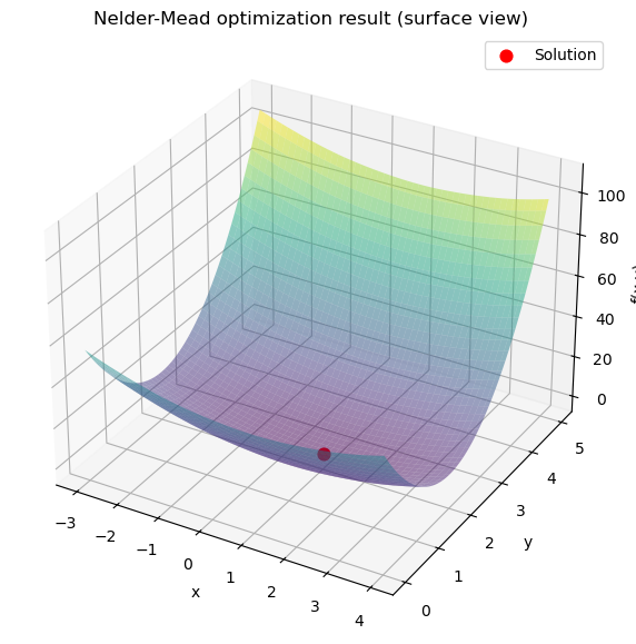
# 3D surface plot
from mpl_toolkits.mplot3d import Axes3D

fig = plt.figure(figsize=(9,7))
ax = fig.add_subplot(111, projection='3d')
ax.plot_surface(X, Y, Z, cmap="viridis", alpha=0.5)
ax.scatter(res_nm.x[0], res_nm.x[1], f_nm(res_nm.x), color="red", s=60, label="Solution")
ax.set_xlabel("x")
ax.set_ylabel("y")
ax.set_zlabel("f(x,y)")
ax.set_title("Nelder-Mead optimization result (surface view)")
ax.legend()
plt.show()

Some final thoughts…

1. Optimization and root finding are related as we could see today. But further conditions must be checked/satisfied (curvature). Optimization is a huge research field, with real world applications!

2. Curve fitting is a form of optimization problem. We are minimizing the errors between a model prediction and data, by numerically manipulating a set of parameters using the optimization algorithm. This is closely-related to training in machine learning!

3. Sometimes, we may not have access to derivatives. Hence, derivative-free methods can be important.