Lecture 10 — Advanced topics I

Based on your exceptional participation in last class, I took your questions home and created this advanced topics class. It’s wonderful to see you actively participating in this class with more complex questions.

Therefore, I decided to review most of your questions and also cover dimensionality reduction techniques. I hope you enjoy this class!

Learning Outcomes

By the end of this lecture, you will be able to:

0. Have the answer for: Is sklearn really useful in real-world applications?

1. Understand K‑Fold Cross‑Validation (CV)

2. Be familiar with Learning Curves in sklearn

3. Understand and identify Overfitting: Model Capacity vs. Score

4. Know the difference between dimensionality Reduction techniques: PCA vs t‑SNE — practical explanations and uses

5. Perform hyperparameter tuning with GridSearchCV

6. Linear decision trees

import numpy as np
import matplotlib.pyplot as plt

from sklearn.model_selection import KFold, train_test_split, LearningCurveDisplay, GridSearchCV, cross_val_score
from sklearn.metrics import mean_squared_error
from sklearn.tree import DecisionTreeRegressor
from sklearn.decomposition import PCA
from sklearn.manifold import TSNE
from sklearn.datasets import load_digits

# Reusable random state
rng = np.random.RandomState(42)

0) SKlearn in the industry

Is this used at all? Looks like it! Let’s take a look in the link below!

https://scikit-learn.org/stable/testimonials/testimonials.html

TLDR:SKlearn is widely used in real applications!

However, big tech companies like Google and Microsoft also develop their own ML packages. Examples are JAX, TensorFlow, LightGBM

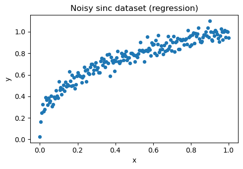
Back to our class… We use a toy dataset/function from previous lectures for regression demos.

X = np.linspace(0, 1, 200).reshape(-1, 1)
y = X[:, 0]**(1/3) + rng.normal(0, 0.05, size=X.shape[0])

plt.figure(figsize=(5,3.5))
plt.scatter(X, y, s=18)
plt.title('Noisy sinc dataset (regression)')
plt.xlabel('x')
plt.ylabel('y')
plt.tight_layout()

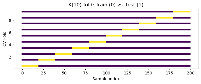
1) Understand K‑Fold Cross‑Validation (CV)

Below we employ simple KFold. We’ll plot which indices belong to train vs test in each fold for our regression dataset.

kf2 = KFold(n_splits= 10)

def plot_kfold_assignments(cv, n_samples):
    plt.figure(figsize=(7,3))

    for i , (tr, te) in enumerate(cv.split(np.arange(n_samples))):
        mask = np.full(n_samples, -1.0)
        mask[tr] = 0.0
        mask[te] = 1.0
        plt.scatter(range(n_samples), [i + 0.5]*n_samples, c=mask, marker='s', s=18, linewidths=0)
    
    plt.xlabel('Sample index')
    plt.ylabel('CV Fold')
    plt.title('K(10)-fold: Train (0) vs. test (1)')
    plt.tight_layout()
                                  

plot_kfold_assignments(kf2, n_samples=len(X))

reg = DecisionTreeRegressor(max_depth=5, random_state=42)
scores = cross_val_score(reg, X, y, cv=kf2, scoring='neg_root_mean_squared_error')
print('k-fold CV RMSE', -scores)
print('Mean RMSE', -scores.mean())

k-fold CV RMSE [0.2323499  0.09238678 0.03926587 0.07719534 0.07433862 0.05981049
 0.06512668 0.05900143 0.05520009 0.13297972]
Mean RMSE 0.08876549227198552

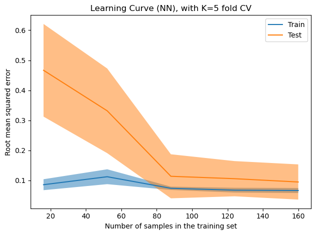
2) Learning Curves (with LearningCurveDisplay)

We plot training score and cross‑validation score vs. the number of training samples, for example, Let’s use a MLPRegressor from the NN class example (Lecture 7).

from sklearn.neural_network import MLPRegressor

reg = MLPRegressor(hidden_layer_sizes=(3,),
                   activation='tanh',
                   solver='lbfgs',
                   alpha=0.5,
                   max_iter=5000,
                   random_state=42




)

kf5 = KFold(n_splits=5)

disp = LearningCurveDisplay.from_estimator(reg,
                                           X,
                                           y,
                                           cv=kf5,
                                           scoring='neg_root_mean_squared_error',
                                           negate_score= True)

plt.title('Learning Curve (NN), with K=5 fold CV')
plt.tight_layout()

3) Overfitting: Capacity vs. RMSE

Overfitting is a common issue in ML. It occurs when the model works extremely well for the training dataset, but it does not generalize well when we do inference in the test/validation sets. Let’s go straight to an example.

We increase model capacity via max_depth of the decision tree and track training RMSE and validation RMSE.
To make the effect clear, we keep the dataset modest so deeper trees can overfit.

X_tr, X_te, y_tr, y_te = train_test_split(X, y, test_size=0.2, random_state=42)

depths = list(range(1, 21))

rmse_train, rmse_val = [], []

for d in depths:
    reg = DecisionTreeRegressor(max_depth=d, random_state=0)
    reg.fit(X_tr, y_tr)
    yhat_tr = reg.predict(X_tr)
    yhat_te = reg.predict(X_te)
    rmse_train.append(np.sqrt(mean_squared_error(y_tr, yhat_tr)))
    rmse_val.append(np.sqrt(mean_squared_error(y_te, yhat_te)))

fig, ax1 = plt.subplots(figsize =(6,4))

ax2 = ax1.twinx()
ax1.plot(depths, rmse_train, marker='o', c='k', label= 'Train RMSE')
ax2.plot(depths, rmse_val, marker='s', c='r', label='Validation RMSE')

ax1.set_xlabel('Tree max_depth (model capacity)')
ax1.set_ylabel('Train RMSE')
ax2.set_ylabel('Validation RMSE')
ax1.set_title('Overfitting: Train vs. Validation RMSE (separate axes)')


lines1, labels1 = ax1.get_legend_handles_labels()
lines2, labels2 = ax2.get_legend_handles_labels()

ax1.legend(lines1 + lines2, labels1 + labels2, loc='upper right')
plt.tight_layout()

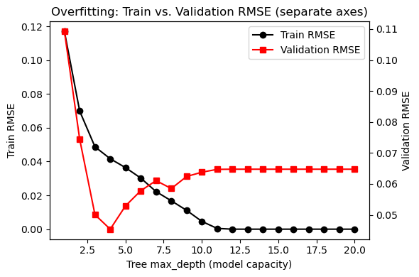
You can see from the red curve that after a certain value of the max_depth, the RMSE actually gets worse, despite the training RMSE decreases! Looking only at the train score can be misleading!

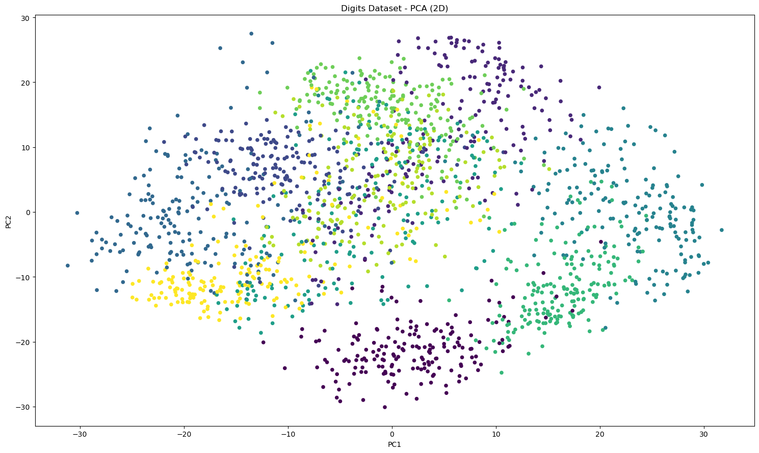
4) Dimensionality Reduction: PCA vs t‑SNE

We focus on representation (not clustering). Both methods map high dimensional data to low dimensions, for visualization purposes. It is beyond the scope of this class to go over all mathematical details of PCA and t-SNE, but I think it’s a good idea to introduce the topic to you all.

PCA — Principal Component Analysis (linear)

• Finds orthogonal directions (principal components) that maximize variance.

• Math (sketch): center data \(X\in\mathbb{R}^{n\times d}\), compute covariance \(\Sigma = \tfrac{1}{n} X^\top X\) PCs are eigenvectors of \(\Sigma\) with eigenvalues giving explained variance

• Properties: linear, fast, global; components are linear combinations of original features

t‑SNE — t‑Distributed Stochastic Neighbor Embedding (nonlinear)

• Builds probability distributions over pairs of points so that nearby points have high probability in high dimensions and (in the map/embedding) in low dimensions.

• Properties: emphasizes local “neighborhoods”; distances between far groups are not meaningful; sensitive to random seed.

Again: Neither PCA nor t‑SNE is a classifier or a clustering algorithm. They are dimensionality reduction techniques.

Trivia: t-SNE was created by the same guy who did fundamental and groundbreaking work in neural networks, Geofrrey Hinton, which was a CMU faculty. Here’s the link to t-sne paper.

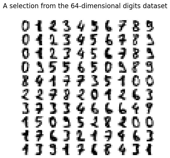
Here, we use the famous digits dataset.

# Example: Digits data 
digits = load_digits()
Xd = digits.data
yd = digits.target

# Display the last digit (# Code source: Gaël Varoquaux) 
# Modified for documentation by Jaques Grobler
# License: BSD 3 clause
# https://scikit-learn.org/1.5/auto_examples/datasets/plot_digits_last_image.html
plt.figure(1, figsize=(3, 3))
plt.imshow(digits.images[-1], cmap=plt.cm.gray_r, interpolation="nearest")
plt.show()

# Authors: The scikit-learn developers
# SPDX-License-Identifier: BSD-3-Clause
fig, axs = plt.subplots(nrows=10, ncols=10, figsize=(6, 6))
for idx, ax in enumerate(axs.ravel()):
    ax.imshow(Xd[idx].reshape((8, 8)), cmap=plt.cm.binary)
    ax.axis("off")
_ = fig.suptitle("A selection from the 64-dimensional digits dataset", fontsize=16)

# PCA (2D)

pca = PCA(n_components = 4 , random_state=0)
Xd_pca = pca.fit_transform(Xd)

plt.figure(figsize=(15, 9))
plt.scatter(Xd_pca[:, 0], Xd_pca[:,1], c = yd, s=20)
plt.title('Digits Dataset - PCA (2D)')
plt.xlabel('PC1')
plt.ylabel('PC2')
plt.tight_layout()

tsne = TSNE(n_components=2, init='pca', learning_rate='auto', perplexity=30, random_state=0)

Xd_tsne = tsne.fit_transform(Xd)
plt.figure(figsize=(15, 9))
plt.scatter(Xd_tsne[:, 0], Xd_tsne[:,1], c = yd, s=20)
plt.title('Digits Dataset - TSNE (2D)')
plt.xlabel('dimension 1')
plt.ylabel('dimension 2')
plt.tight_layout()

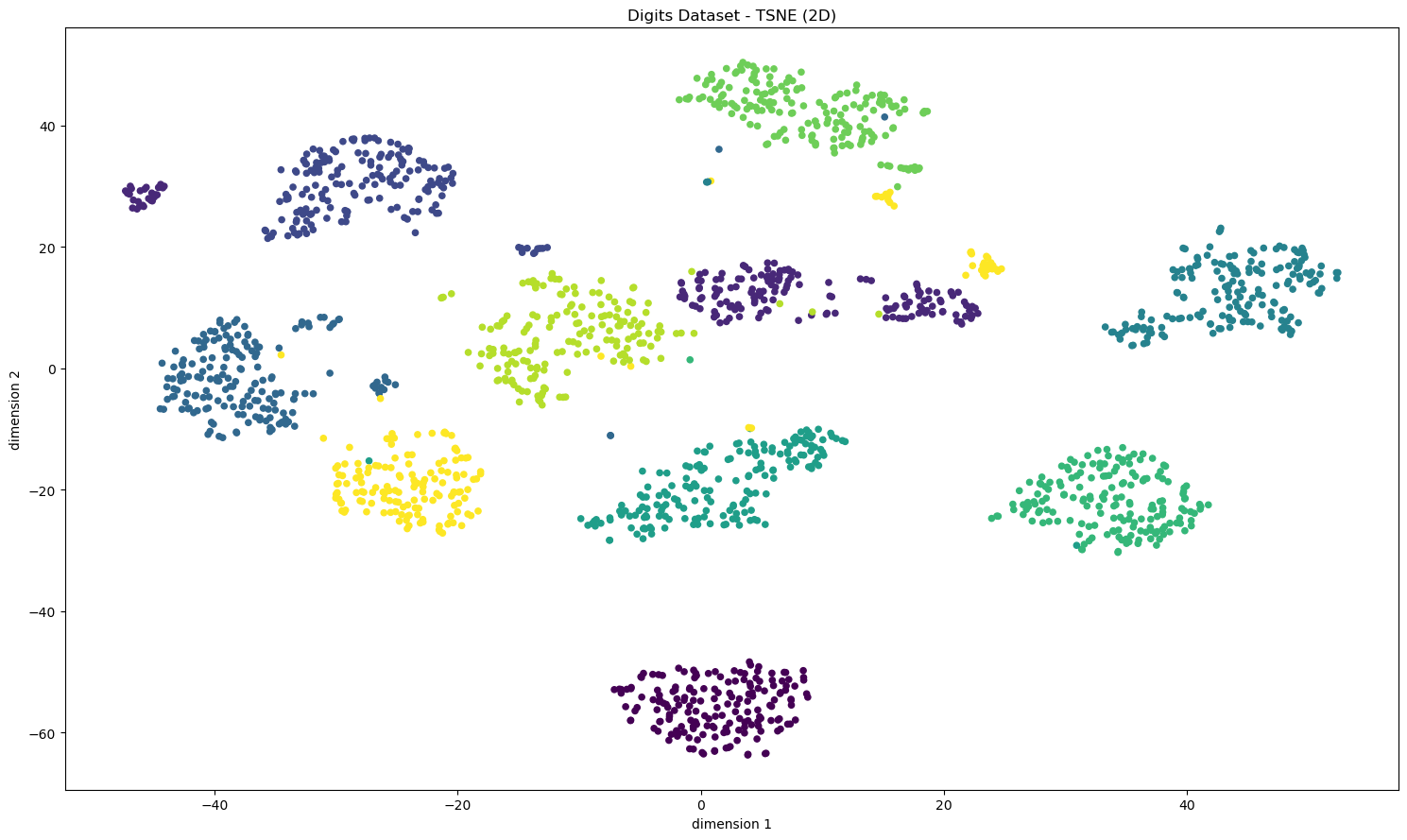
Some interesting stuff on PCA and T-SNE:

• Principal Component Analysis, explained visually

• A Visual and Overly Simplified Guide to PCA

• Interactive publication on t-sne by Google researchers

Ok, but what now?

• Color encodes the ground‑truth digit (only for interpretation).

• PCA: linear projection; some digits overlap because the underlying separation is nonlinear.

• t‑SNE: same digits tend to form “islands”.

Practical tips:

• Start with PCA: It’s quick, and has linear structure; inspect explained variance to choose dimensions.

• Use t‑SNE for local manifold structure; try a few perplexity values (e.g., 5–50). Fix random_state for reproducibility.

PCA vs t‑SNE — key differences

Aspect	PCA	t‑SNE
Type	Linear projection	Nonlinear embedding
Preserves	Global variance directions	Local neighborhoods
Distances between far groups	Meaningful (linear)	Not meaningful
Speed / scale	Fast, scalable	Slower; tune perplexity
Main knobs	n_components	perplexity, learning_rate, initialization
Use cases	Compression, denoising, quick structure check	Visualizing clusters/manifolds; exploratory analysis

5) Hyperparameter Tuning with GridSearchCV

This was another question from previous class: “Can we do better when coming up with the selection of the hyperparameters”.

Yup! Let’s see an example.

We tune a DecisionTreeRegressor on our toy dataset, searching over max_depth and min_samples_leaf using KFold CV.

param_grid = {

    'max_depth': [2, 3, 4, 5, 6],
    'min_samples_leaf': [1, 2, 4, 8]


}

base = DecisionTreeRegressor(random_state=0)

cv = KFold(n_splits=5)

gcv = GridSearchCV(base, param_grid, cv = cv, scoring = 'neg_root_mean_squared_error')
gcv.fit(X, y)

print('Best parameters:', gcv.best_params_)
print('Best CV RMSE:', -gcv.best_score_)

Best parameters: {'max_depth': 4, 'min_samples_leaf': 2}
Best CV RMSE: 0.09441459329669424

6) Linear decision trees

It turns out that when working with tree, the decision on/when to split doesn’t have to be necessarily a constant value (standard decision trees). They can be linear relationships, which brings enormous flexibility to ML regression models.

Linear decision trees are not natively available in SKLearn, but there is a package called linear-tree based on Sklearn that allows the ML modeling of linear decision trees.

In our department, prof. Laird and his PhD students work quite extensively with linear decision trees, embedding them in optimization problems. A package called OMLT - Optimization and Machine Learning Toolkit developed together with collaborators from the Imperial College allows to “translate” these ML trees into an optimization modeling language called Pyomo.

Why is this useful?

• We bridge ML and Optimization theory together. We can express optimization problems with ML models/surrogates!

• Let’s take a look at this paper from one of Prof. Laird’s students

• These problems can be represented as mixed-integer programming problems. You’ll see more details on the next mini class!

Summary

• KFold cross validation CV is a powerful tool to perform model selection.

• Learning curves can show the effect of training dataset size.

• Overfitting can be identified, among several possible tests, as low training RMSE but rising validation RMSE as model capacity increases.

• PCA vs t‑SNE: linear global variance vs nonlinear local neighborhoods; choose based on your goal.

• GridSearchCV wraps CV to select hyperparameters using your familiar models from previous classes!