Final Class — Advanced Topics II - Clustering, Scientific ML (PINNs & Neural ODEs) concepts, and Course Review#
Learning Outcomes#
Explain the K‑means objective \(J\) and the basic assign/update steps.
Use scikit‑learn to run K‑means; interpret inertia.
Understand the big picture of Scientific ML with PINNs and Neural ODEs.
Review the main points from each lecture of the course.
1) K‑means clustering#
K-means clustering is the simplest clustering algorithm available. Let’s take a look at it’s high level functionality. How it works and how can we make use of it.
Objective function#
Choose \(K\) clusters. Find centroids \(\{\mu_1,\dots,\mu_K\}\) and assignments \(c(i)\in\{1,\dots,K\}\) that minimize
Intuition: \(J\) sums squared distances from each point to its cluster centroid. Minimizing \(J\) makes clusters compact.
Pros / Cons#
Pros: fast; simple; effective for spherical, well‑separated clusters.
Cons: must choose \(K\); sensitive to feature scaling and outliers; struggles with non‑spherical shapes or very different densities.
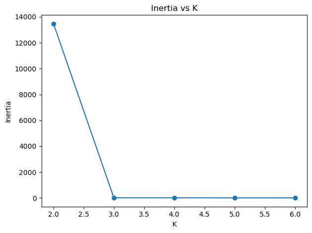
Main metric we usually employ in sklearn
Inertia (
kmeans.inertia_): value of \(J\) (also called within‑cluster sum of squares). Lower is better but always decreases as \(K\) grows.
A simple example#
Let’s generate a simple dataset, make_blobs sweep a few \(K\), look at inertia, then visualize one fit.
import numpy as np

import matplotlib.pyplot as plt
from sklearn.datasets import make_blobs
from sklearn.cluster import KMeans


X, _ = make_blobs(n_samples= 800, centers=3, cluster_std=0.1, random_state=42)


Ks = range(2,7)
inertias = []

for k in Ks:
    kmeans = KMeans(n_clusters=k, n_init='auto', random_state=0).fit(X)
    inertias.append(kmeans.inertia_)

plt.figure()
plt.plot(list(Ks), inertias, '-o')
plt.xlabel("K")
plt.ylabel("Inertia")
plt.title("Inertia vs K")
plt.tight_layout()
kmeans = KMeans(n_clusters=3, n_init='auto', random_state=0).fit(X)
labels = kmeans.labels_
centers = kmeans.cluster_centers_

plt.figure()
plt.scatter(X[:,0], X[:,1], c=labels, s=15, alpha=0.9)
plt.title("Our last plot!!!!!")
plt.xlabel("x1")
plt.ylabel("x2")
plt.tight_layout()
print(kmeans.labels_)
[1 1 2 2 2 1 0 0 2 1 0 2 0 2 0 1 1 0 0 1 2 2 1 1 0 2 0 0 1 0 0 1 0 1 0 2 0
 1 2 2 2 2 0 0 0 0 1 0 1 2 1 0 2 1 1 0 2 2 1 1 1 2 1 2 1 0 0 1 0 2 1 0 2 1
 2 1 0 1 0 0 1 1 0 2 2 2 0 1 0 0 0 1 1 2 1 1 0 1 0 1 2 0 0 1 1 2 2 2 2 1 1
 0 2 0 2 0 0 1 0 2 0 2 2 1 0 0 2 0 1 2 1 1 0 2 2 1 0 1 0 0 2 0 0 1 1 0 2 0
 2 0 2 0 0 1 0 2 1 1 2 0 1 0 2 0 1 0 1 1 1 2 2 1 1 2 0 0 2 2 2 2 0 2 0 0 1
 0 2 2 2 2 0 0 1 1 1 0 0 0 1 2 1 2 0 1 0 2 2 2 2 0 1 2 1 2 2 2 1 0 0 2 0 1
 1 0 2 0 0 1 0 1 0 1 0 2 0 1 2 2 0 1 1 2 2 2 2 1 1 2 0 2 0 0 2 2 1 2 2 1 1
 0 2 0 1 0 2 1 0 2 2 1 0 2 2 2 0 0 0 0 0 0 2 1 0 0 0 2 1 0 2 0 2 2 1 0 0 0
 2 2 2 2 2 0 0 1 1 0 2 1 1 0 2 2 0 0 2 0 2 2 2 0 2 1 2 0 0 1 2 0 1 1 0 0 2
 2 2 1 0 1 1 1 0 0 2 1 2 0 0 2 1 2 1 0 1 1 1 0 2 0 1 2 1 0 1 0 0 1 1 0 2 2
 2 0 1 0 1 0 1 0 1 0 1 0 2 2 0 1 0 2 1 0 0 1 2 0 1 2 2 0 1 0 2 1 1 0 0 0 1
 1 0 2 0 1 1 2 2 1 2 0 2 2 1 1 2 2 2 2 0 2 2 2 0 1 2 2 2 1 0 1 0 0 0 1 1 0
 0 1 1 0 0 1 1 0 2 1 1 0 0 2 1 0 2 2 1 0 2 2 0 0 0 2 2 0 0 0 2 1 0 2 1 1 0
 1 2 0 0 0 1 0 1 1 1 0 1 2 0 1 0 0 1 1 0 1 1 1 1 1 2 1 1 0 0 0 1 1 2 1 2 1
 0 2 0 1 2 2 2 2 0 1 1 0 1 2 1 1 0 2 2 2 2 2 1 1 1 0 0 2 2 1 0 2 0 1 1 2 2
 0 0 2 1 1 0 2 1 2 1 0 2 2 1 2 2 2 1 0 2 2 1 2 2 1 2 2 2 2 1 2 1 0 1 2 0 1
 1 0 0 2 0 1 0 2 0 0 1 2 1 2 2 2 0 2 1 2 0 0 2 0 2 2 2 0 1 0 2 2 2 1 2 1 1
 2 1 0 1 1 2 1 2 2 0 0 0 1 0 2 1 2 2 2 1 2 1 1 1 0 2 2 1 0 1 0 0 1 0 1 0 1
 0 2 1 2 2 1 1 2 1 0 2 0 2 2 1 0 1 1 2 0 0 0 2 1 1 1 0 2 2 2 2 2 1 0 1 2 1
 2 0 2 1 1 1 1 2 1 0 2 0 1 1 0 1 2 0 1 0 2 1 2 0 1 1 0 2 1 1 2 0 1 1 1 1 2
 0 0 2 0 1 2 0 2 2 1 2 2 1 0 0 0 1 1 0 1 2 0 2 2 2 0 1 2 2 2 1 2 0 2 1 2 1
 1 0 1 0 0 0 1 0 2 0 0 1 2 1 1 1 1 0 0 1 2 1 0]
2) Scientific Machine Learning (SciML) — PINNs & Neural ODEs (simplified)#
2.1 Big idea#
Blend first‑principles (balances, kinetics, transport) with learning for models that are data‑efficient and physics‑consistent.
2.2 PINNs (Physics Informed Neural Networks)#
Train a neural network \(x_\theta\) to fit data and approximately satisfy some physics you specify (ODE/DAE/PDE). One simple training objective:
where \(\mathcal{F}[\cdot]\) is any physics residual you choose.
2.3 Neural ODEs (continuous‑depth networks)#
Parameterize a vector field and integrate it:
Think of residual networks with step size \(\Delta t \to 0\); training uses differentiable ODE solvers / adjoint ideas.
Please take a look at the slides I presented to you. They are available on Canvas.
3) Course Review — main points by lecture#
These bullets follow the structure on the course website. Let’s go over them one-by-one.
Lecture 1 — Python for Numerical Methods (essentials).
Motivation for Python; NumPy arrays and vectorization; control flow; plotting.
ChemE‑flavored examples (mass balances, EOS, batch reactor), building coding habits.
Lecture 2 — Nonlinear systems: root finding.
Bracketing (bisection) vs open (Newton/secant) methods; stopping criteria and convergence.
Extending to systems with Jacobians; practical pitfalls and scaling.
Lecture 3 — Optimization (unconstrained & constrained).
Objective + constraints; first/second‑order optimality ideas.
Curve‑fitting (SSE) and
scipy.optimize.minimizewith bounds/constraints.
Lecture 4 — ODEs (I).
IVPs; explicit/implicit integrators; stability vs accuracy;
scipy.integrate.solve_ivp.Events/forcing and step‑size effects.
Lecture 4/5 — ODEs (II).
Larger ODE systems; modeling patterns; diagnostics and engineering context; nullclines; stability.
Lecture 6 — ML I (intro & workflow).
Train/validation/test; feature considerations; linear regression; decision trees; “pipeline” mindset.
Lecture 7 — ML II (regression: neural networks).
MLP architecture; activations; optimization; regularization; over/under‑fitting.
Lecture 8 — ML II (regression: Gaussian processes).
Kernels (RBF/Matérn/periodic); posterior mean + uncertainty; marginal likelihood; small‑data strengths.
Lecture 9 — ML III (classification).
Decision boundaries; calibration; imbalanced data caveats; metrics beyond accuracy.
Lecture 10 — Advanced topics / review.
Model selection; validation tools in SKlearn.
A final note from me…#
It’s been a pleasure teaching this class. I’m proud of your progress and curiosity, and I wish each of you the very best as you carry these tools into your careers. Keep building, keep questioning, and keep learning!