Lecture 4 — Ordinary Differential Equations (ODEs)#
Learning outcomes#
Recognize when ODE integrators are needed and the assumptions behind (Initial Value Problems) IVPs.
Derive the Forward Euler method from a Taylor Series Expansion (TSE).
Understand the idea of Runge–Kutta (RK) methods (RK45).
Implement a simple Euler integrator and compare against analytical solutions.
Use
scipy.integrate.solve_ivpand its useful functionalities (events, forcing functions).
1) Motivation in chemical engineering#
A few examples:
Kinetics: batch reactor decay/growth rates \(dC/dt = r(C,t)\).
Bioprocesses: cell growth (logistic/Monod), substrate consumption.
Reactors: CSTR components and energy balances, residence time effects.
Control: dynamic response to set point/step changes.
Transport Phenomena: Mass/Heat/Momentum transfer can be modeled using ODE systems.
We typically know an initial condition \(y(t_0)=y_0\) and a differential equation (or equations) \(y'(t)=f(t,y)\);
we seek \(y(t)\) for \(t\in[t_0,t_f]\).
2) Derivation — Forward Euler from TSE#
Start with the initial value problem (IVP)
The Taylor expansion of \(y(t)\) at \(t_n\) is
in which \(h=t_{n+1} - t_{n}\) and since \(y'(t_n) = f(t,y)\), we have
Dropping higher-order terms gives the Euler update formula
3) Runge–Kutta (RK) idea (overview)#
Goal: improve accuracy by sampling \(f\) within the step. This is achieved by doing the algebra above, but keeping high order terms from TSE.
Classical RK4 (fixed step) uses four stages
and the update
The idea is similar to Euler’s (which is also known as… \(1^{st}\) order Runge-Kutta method), it just uses higher order terms in the TSE. The math is a bit tedious but if you are interested you can take a look online.
Adaptive RK45 (Dormand–Prince) (used in solve_ivp(method='RK45')) estimates the local error by embedding a 4th- and 5th-order pair and automatically adjusts \(h\) to meet tolerances (rtol, atol).
4) A minimal Euler integrator (fixed step)#
How the code looks like for the simplest integrator (Euler / \(1^{st}\) order RK)? Here’s an example!
import numpy as np


def euler(f, t_span, y0, h):

    """
    A very simple Euler integrator (a.k.a 1st order Runge-Kutta)


    Inputs
    -------
    f: function
        The function that represents the RHS f(t, y).
    t_span: (t0, tf) tuple
        Integration interval
    y0: float
        Initial condition at t0.
    h: float
        Fixed step size

    Returns
    -------

    t: np.ndarray
        Time points
    Y: np.ndarray
        Solution values at each time.


    """

    t0, tf  = float(t_span[0]), float(t_span[1])

    t = np.append(np.arange(t0, tf, h), tf)


    Y = np.empty((t.size, ))


    Y[0] = y0


    for i in range(t.size - 1):

        Y[i + 1] = Y[i] + h * (f(t[i], Y[i]))

    return t, Y
5) Example 1 — Batch reactor first-order decay#
Let’s look at first-order kinetics in a batch reactor. This example has an analytical solution. Hence, we will be able to check the accuracy of our integrator :)
The model is conceptually simple, defined as
The analytical solution is given as $\(\,C(t)=C_0 e^{-kt}.\)$
Let’s compare Euler to the exact solution and to scipy.integrate.solve_ivp at the default method (RK45).
import numpy as np
import matplotlib.pyplot as plt
from scipy.integrate import solve_ivp


# Constants
C0, k = 1.0, 0.6

# Our ODE
def batch_reactor(t, C):
    return -k * C

# Euler call
step = 0.15
t_eu, C_eu = euler(batch_reactor, (0.0, 8.0), C0, h=step)

# Exact solution over a range
t_exact = np.linspace(0, 8, 200)
C_exact = C0*np.exp(-k*t_exact)

# RK45
sol = solve_ivp(batch_reactor, (0.0, 8.0), [C0], method='RK45', rtol=1e-8, atol=1e-10, dense_output=True)
t_rk = np.linspace(0, 8, 200)
C_rk = sol.sol(t_rk)[0]

plt.figure(figsize=(7,4.5))
plt.plot(t_exact, C_exact, label='Exact', lw=2)
plt.plot(t_eu, C_eu, 'o-', label=f'Euler {step:.3f}')
plt.plot(t_rk, C_rk, '--', label='RK45 (solve_ivp)')
plt.xlabel('t')
plt.ylabel('C(t)')
plt.title('First-order decay: Euler vs RK45 vs Exact')
plt.grid(True); plt.legend(); plt.show()
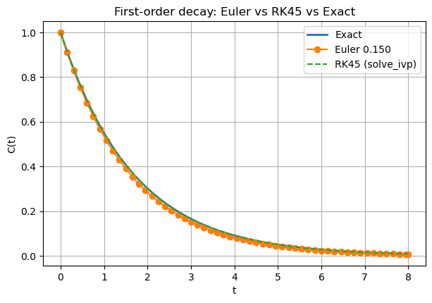
If we reduce the step size \(h\), Euler’s method gets closer to both the analytical solution and RK45.
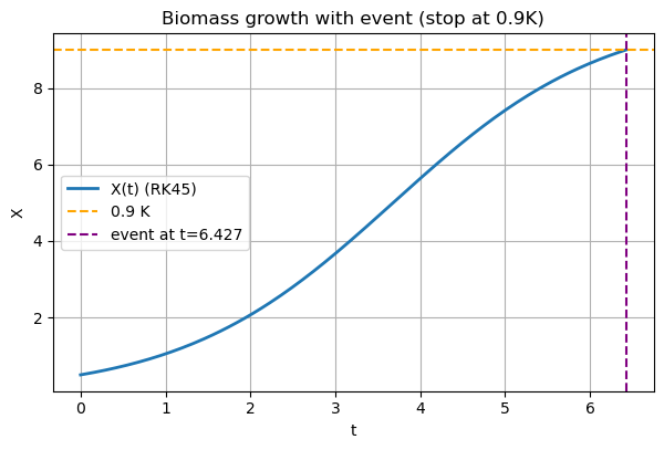
6) Example 2 — Events (stop when some desired threshold/condition is reached)#
Let’s assume that a generic bioprocess is modeled after the following ODE:
\(r, K\) are constants specific to the biomass that is increasing, \(X\). We want to stop the integration when \(X(t)\) hits \(0.9K\) (an event).
In solve_ivp, we achieve this by setting the keyword argument event.terminal = True and event.direction = +1 (rising).
# Our constants and initial condition
r, K, X0 = 0.8, 10.0, 0.5

def bioprocess(t, X):
    dXdt = r * X * (1.0 - X / K)
    return dXdt

def hit_90pct(t, X):
    # event when X - 0.9K = 0 (crossing upward)
    return np.array(X) - 0.9*np.array(K)

hit_90pct.terminal = True
hit_90pct.direction = +1.0


sol = solve_ivp(bioprocess,
                (0.0, 20.0),
                [X0],
                events=hit_90pct,
                rtol=1e-8,
                atol=1e-10,
                dense_output=True)


t_plot = np.linspace(0, sol.t_events[0][0], 200) if len(sol.t_events[0])>0 else np.linspace(0, 20, 200)
X_plot = sol.sol(t_plot)[0]

import matplotlib.pyplot as plt
plt.figure(figsize=(7,4.2))
plt.plot(t_plot, X_plot, lw=2, label='X(t) (RK45)')


if len(sol.t_events[0])>0:
    t_hit = sol.t_events[0][0]
    plt.axhline(0.9*K, color='orange', ls='--', label='0.9 K')
    plt.axvline(t_hit, color='purple', ls='--', label=f'event at t={t_hit:.3f}')
plt.xlabel('t'); plt.ylabel('X')
plt.title('Biomass growth with event (stop at 0.9K)')
plt.grid(True); plt.legend(); plt.show()
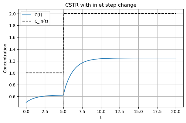
7) Example 3 — Forcing function (CSTR concentration step change)#
One more example. In this CSTR, we can manipulate its inlet concentration \(C_{in}\). This is not uncommon in process control, for example. The system is modeled as:
Let \(C_{\text{in}}(t)=1\) for \(t<5\) and \(C_{\text{in}}(t)=2\) for \(t\ge 5\).
import numpy as np, matplotlib.pyplot as plt
from scipy.integrate import solve_ivp

F, V, k = 1.0, 2.0, 0.3
C0 = 0.5
t_span = [0.0, 20.0]


def C_in(t):
    # This makes the concentration change when t >= 5
    return 1.0 if t < 5.0 else 2.0

def cstr(t, C):
    # Simple CSTR balance

    dCdt = (F/V)*(C_in(t) - C) - k*C
    return dCdt

# Let's solve this with dense_output=True so we can plot the solution easily
sol = solve_ivp(cstr, t_span, [C0], dense_output=True)

print(sol)
  message: The solver successfully reached the end of the integration interval.
  success: True
   status: 0
        t: [ 0.000e+00  1.380e-01 ...  1.942e+01  2.000e+01]
        y: [[ 5.000e-01  5.131e-01 ...  1.250e+00  1.250e+00]]
      sol: <scipy.integrate._ivp.common.OdeSolution object at 0x10791f8c0>
 t_events: None
 y_events: None
     nfev: 98
     njev: 0
      nlu: 0
Let’s see if this is working!
t_grid = np.linspace(0, 20, 300)
C = sol.sol(t_grid)[0]
Cin = np.array([C_in(ti) for ti in t_grid])
plt.figure(figsize=(7,4.2))
plt.plot(t_grid, C, label='C(t)')
plt.plot(t_grid, Cin, 'k--', label='C_in(t)')
plt.axvline(5.0, color='grey', ls=':', lw=1)
plt.xlabel('t'); plt.ylabel('Concentration')
plt.title('CSTR with inlet step change')
plt.grid(True); plt.legend(); plt.show()
ha ha!
8) Practice problems you might get asked in your HW…#
Derive Euler from TSE; implement and test on a known solution; study step-size effects.
Use
solve_ivpwitheventsto detect and stop at thresholds (e.g., safety limits in a chemical reactor).Model a forced system (e.g., CSTR) with time-dependent inputs.
Explore
method='RK45'(adaptive) andmethod='BDF'(for stiff problems).